[Primer] Fractal Dimension in EEG Signal Analysis

This primer provides the fractal dimension background for the Fractals Properties of EEG During Motor Imagery project. For EEG fundamentals and the ERD/ERS paradigm referenced throughout, see the companion primer [Primer] Brain-Computer Interfaces Using EEG.

Classical signal processing treats biosignals as the sum of sinusoidal components. But biological signals are not stationary, not periodic, and not well-described by their frequency content alone. The brain, heart, and other physiological systems are inherently non-linear, and their outputs reflect that complexity. Fractal dimension is a tool from non-linear dynamics that quantifies a different property of a signal: how complex, irregular, or self-similar it is over time. This primer covers what fractal dimension is, how it is computed for a time series, and why it is useful for EEG analysis.

---

What Is a Fractal?

A fractal is a geometric object that displays self-similarity across scales: zooming in on any part of it reveals structure similar to the whole. The term was coined by Benoit Mandelbrot, who observed that natural phenomena such as coastlines, clouds, and trees are better described by fractals than by smooth Euclidean geometry.

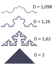
The key property of a fractal is that it does not fit neatly into an integer dimension. A straight line is one-dimensional, a filled square is two-dimensional. A fractal curve that is highly convoluted occupies more space than a line but does not fill the plane, so its dimension is somewhere between 1 and 2. This non-integer value is the fractal dimension \(D\).

Formally, for a self-similar object that can be subdivided into \(N\) copies each scaled by a ratio \(r\):

\[D = \frac{\log N}{\log(1/r)}\]

For a Koch snowflake-type curve at each iteration, the curve is divided into 4 copies each scaled by 1/3, giving \(D = \log 4 / \log 3 \approx 1.26\). Smoother curves approach \(D = 1\); space-filling curves approach \(D = 2\).

---

Fractal Dimension of a Time Series

A time series such as an EEG recording is a sequence of scalar values over time, not a geometric object in the usual sense. But the same underlying idea applies: a highly irregular, jagged signal with fine-scale fluctuations at all timescales occupies more of the time-amplitude plane than a smooth one. The fractal dimension of a time series quantifies this irregularity.

Several methods exist to estimate the fractal dimension of a time series. Among these, Higuchi’s algorithm (Higuchi, 1988) is widely used in EEG analysis because it is computationally efficient, applies directly to the raw time series without embedding, and does not require stationarity.

---

Higuchi’s Algorithm

Given a discrete time series \(X(1), X(2), \ldots, X(N)\), Higuchi’s algorithm estimates fractal dimension by examining how the length of the series scales with the resolution at which it is measured.

Step 1: Construct sub-series at different intervals

For a time interval \(k\) and an initial time \(m\) (\(1 \leq m \leq k\)), define the sub-series:

\[X_m^k: \; X(m), \; X(m+k), \; X(m+2k), \; \ldots, \; X\!\left(m + \left\lfloor\frac{N-m}{k}\right\rfloor k\right)\]

This downsamples the original series to every \(k\)-th point, starting at offset \(m\).

Step 2: Compute the length of each sub-series

The length \(L_m(k)\) of the sub-series \(X_m^k\) is:

\[L_m(k) = \frac{1}{k} \left[ \sum_{i=1}^{\lfloor(N-m)/k\rfloor} \left| X(m+ik) - X(m+(i-1)k) \right| \right] \cdot \frac{N-1}{\lfloor(N-m)/k\rfloor \cdot k}\]

The normalization factor \((N-1) / (\lfloor(N-m)/k\rfloor \cdot k)\) ensures fair comparison across sub-series of different lengths.

Step 3: Average over all initial offsets

For each interval \(k\), average the lengths across the \(k\) possible initial offsets:

\[L(k) = \frac{1}{k} \sum_{m=1}^{k} L_m(k)\]

Step 4: Estimate the fractal dimension by log-log regression

For a fractal process, the curve length scales as a power law with the interval:

\[L(k) \propto k^{-D}\]

Taking logarithms:

\[\log L(k) = -D \cdot \log k + \text{const}\]

The fractal dimension \(D\) is estimated as the negative slope of the linear regression of \(\log L(k)\) against \(\log k\), computed over a range of interval values (typically \(k = 1, 2, \ldots, k_{\max}\)).

The choice of \(k_{\max}\) affects the estimate. Common values range from 5 to 10 for EEG, depending on sampling rate and signal length.

---

Interpreting Fractal Dimension in EEG

For a one-dimensional time series, Higuchi’s FD takes values in the range \([1, 2]\):

• Low FD (close to 1): the signal is smooth and regular, with small-amplitude, slowly-varying fluctuations. Low complexity.
• High FD (close to 2): the signal is highly irregular and jagged, with significant fluctuations at all timescales. High complexity.

FD range	Signal character	Physiological interpretation
1.0 – 1.3	Smooth, low-frequency dominated	Highly synchronized neural activity (e.g., epileptic seizure, deep sleep)
1.3 – 1.7	Intermediate irregularity	Normal waking EEG; motor imagery states
1.7 – 2.0	Highly irregular, broadband	Active, desynchronized cortical state

Intuitively, when the brain is at rest, many neurons oscillate together in large synchronized rhythms (high-amplitude, low-frequency waves), producing a smoother signal with lower FD. When the brain is actively processing information or engaged in a motor task, neural populations desynchronize, producing a more complex and irregular signal with higher FD.

This is consistent with the concept of event-related desynchronization (ERD): when a motor imagery task begins, the mu and beta rhythms over the sensorimotor cortex decrease in power (ERD), and the EEG becomes more irregular. This should correspond to an increase in fractal dimension.

---

Relationship Between FD and ERD/ERS

ERD quantifies the relative change in band-limited power during a cognitive event compared to a pre-event baseline. FD quantifies the overall complexity of the broadband signal. The two are related but distinct:

• ERD is computed within a specific frequency band (e.g., mu: 8-13 Hz, beta: 18-26 Hz). It tells you how much synchronized oscillatory activity in that band has changed.
• FD is computed on the raw or band-filtered signal and reflects its aggregate irregularity across all timescales captured by the signal.

A natural question is whether these two measures covary during motor imagery: specifically, whether the peak of ERD (maximum power suppression) corresponds in time to a minimum in FD (maximum reduction in complexity). Counterintuitively, ERD peak corresponds to FD minimum, not maximum.

The reason is that ERD is a power suppression: the dominant oscillatory rhythm disappears. When a strong, regular rhythm is suppressed, the residual signal loses a dominant periodic component, becoming in a sense less structured in the frequency domain. But in the temporal domain measured by Higuchi’s FD, a signal dominated by one strong oscillatory frequency is actually more regular (lower FD) than truly broadband noise. When the mu rhythm is present and dominant, the signal has a strong periodic structure and relatively low FD. When ERD occurs and the mu rhythm is suppressed, the signal becomes more variable in an irregular, non-oscillatory way, but since the regular oscillation has been replaced by lower-amplitude, less organized activity, the complexity measured by FD can decrease.

In practice, the relationship between ERD and FD depends on the signal frequency band and the dynamics of the transition. In the study this primer supports, the global minimum in FD across the trial aligned with the peak of ERD in the spectral-temporal map, suggesting that the two measures track the same underlying neural event, just from complementary perspectives.

For a detailed account of ERD/ERS quantification, see the [Primer] Brain-Computer Interfaces Using EEG.

---

Why Use FD Alongside ERD in EEG?

FD and ERD answer different questions about the same signal:

Property	ERD/ERS	Fractal Dimension
What it measures	Band-limited power change relative to baseline	Overall signal complexity / irregularity
Frequency specificity	Band-specific (mu, beta, etc.)	Broadband aggregate
Computational model	Linear (spectral power)	Non-linear (scaling law)
Sensitivity to	Oscillatory synchronization	Structure at all timescales

Using FD alongside spectral methods provides a non-linear complement to conventional frequency-band analysis. It can reveal changes in signal structure that are not captured by power alone, and it is particularly useful for detecting state transitions, such as the onset of motor imagery, that manifest across the full frequency spectrum of the EEG.

---

Summary

Fractal dimension is a single scalar index of signal complexity derived from how the measured length of a time series scales with resolution. Higuchi’s algorithm estimates it efficiently and reliably from short EEG epochs without requiring signal stationarity. In the context of motor imagery EEG, FD tracks the same underlying cortical event as ERD: both reach their extremum at the moment of peak motor cortical engagement. This synchronization between a spectral measure (ERD) and a non-linear complexity measure (FD) supports the use of fractal analysis as a complementary tool for understanding and decoding brain states in BCI applications.

References

- Approach to an irregular time series on the basis of the fractal theoryPhysica D: Nonlinear Phenomena, 1988