[Primer] Level Set Methods for Image Segmentation

This post explains the Level Set method as used in the FAZSEG project, which applies DRLSE to segment the Foveal Avascular Zone boundary in retinal OCT-A images. See the project page for the specific implementation details and results on real clinical data.

The Level Set method is a numerical technique for tracking the evolution of curves and surfaces. Rather than explicitly tracking boundary points, it embeds the boundary as the zero contour of a higher-dimensional function, making it naturally capable of handling topological changes such as splits and merges.

Conceptual Visualization

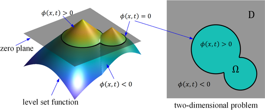
Imagine a mountainous 3D landscape completely submerged underwater. If the water level drops, the peaks of the mountains will eventually break the surface. The shoreline—where the water meets the land—is a 2D closed curve. If we move the 3D landscape up or down, this 2D shoreline changes shape. It might expand, shrink, or even split into two separate islands if a valley emerges.

In this analogy:

• The 3D landscape is the Level Set Function, denoted as $\phi(x, y, t)$.
• The water surface is the zero level, where height = 0.
• The shoreline is our contour or boundary, mathematically defined as the zero level set: $C(t) = {(x,y) \mid \phi(x,y,t) = 0}$.

Instead of explicitly tracking the points of the 2D shoreline (which is difficult when it splits or merges), the Level Set Method evolves the entire 3D landscape $\phi$. The 2D boundary is then simply extracted by finding where $\phi = 0$.

Iteratively Achieving the Boundary of an Object

How does this expanding/shrinking curve “know” where to stop to segment an image? In image processing, the speed function $F$ is tied to the image gradient (edges). We define an edge indicator function $g$, typically formulated as (Osher & Sethian, 1988):

\[g = \frac{1}{1 + \lvert\nabla I\rvert^2}\]

where $I$ is the image intensity. This gives two key behaviors:

• In flat regions (no edges), $\lvert\nabla I\rvert \approx 0$, so $g \approx 1$, the contour moves fast.
• At object boundaries (strong edges), $\lvert\nabla I\rvert$ is large, so $g \approx 0$, the contour stops.

The iterative process proceeds as follows:

1. Initialize: A starting contour is drawn inside or outside the object (e.g., a small circle). $\phi$ is initialized as a 3D cone/bowl representing this circle at zero.
2. Compute Forces: The algorithm looks at the image underneath the contour. If $g \approx 1$, it applies an outward force.
3. Evolve $\phi$: The Hamilton-Jacobi equation updates $\phi$ for a small time step $\Delta t$, shifting the 3D surface.
4. Extract Zero Level Set: The new boundary $C(t+\Delta t)$ is implicitly found where the updated $\phi = 0$.
5. Convergence: Steps 2–4 repeat. The contour expands rapidly through uniform regions but slows to a halt when it hits the high-gradient boundary of the object ($g \to 0$).

Distance Regularization (Li et al., 2010)

While Osher and Sethian’s formulation is elegant, it has a numerical flaw during iteration: as $\phi$ evolves, the 3D landscape can become extremely steep or flat near the zero level set, causing severe numerical inaccuracies.

Traditionally, this was fixed by periodically re-initializing $\phi$ to be a Signed Distance Function (SDF)—a specific shape where the slope is uniform everywhere ($\lvert\nabla \phi\rvert = 1$). However, re-initialization is computationally expensive and moves the zero level set, creating artifacts.

(Li et al., 2010) solved this by introducing Distance Regularized Level Set Evolution (DRLSE). Instead of manually fixing $\phi$, they added a mathematical penalty directly into the evolution equation to force $\phi$ to maintain the SDF property automatically. They defined an energy functional with a distance regularization term $R_p(\phi)$:

\[R_p(\phi) = \int_\Omega p(\lvert\nabla \phi\rvert) \, dx\]

where $p(s) = \frac{1}{2}(s-1)^2$. This term acts like a “spring” on the gradient, if the slope $\lvert\nabla \phi\rvert$ deviates from $1$, this energy increases. By minimizing the total energy, the level set equation becomes:

\[\frac{\partial \phi}{\partial t} = \mu \, \text{div} \left( d_p(\lvert\nabla \phi\rvert) \nabla \phi \right) + \text{External Image Forces}\]

Because of this regularization, the 3D landscape of $\phi$ smoothly maintains a slope of $1$ near the zero level set. The DRLSE algorithm completely eliminates the need for periodic re-initialization, making the iterative boundary-finding process vastly more stable, faster, and easier to implement.