FAZSEG
Automatic Foveal Avascular Zone Segmentation Using Hessian-Based Filter and U-Net Deep Learning Network
This work as been published at 8th International Conference on the Development of Biomedical Engineering in Vietnam (BME2020). Github’s repo
Introduction
Optical Coherence Tomography Angiography (OCTA) has emerged as a rapid, high-resolution, and non-invasive imaging modality for generating volumetric angiographic images. It is a highly promising tool for evaluating and detecting common retinal diseases, including age-related macular degeneration, diabetic macular edema, and choroidal neovascularization (de Carlo et al., 2015; Virgili et al., 2015; Jia et al., 2014). A critical biomarker in assessing these conditions is the foveal avascular zone (FAZ), as its accurate extraction is vital for detecting vascular diseases that affect retinal microcirculation.
Historically, researchers have relied on traditional computer vision algorithms from simple morphological algorithm (Díaz et al., 2019) to advanced active contours algorithm such as Generalized Gradient Vector Flow (GGVF) (Lu et al., 2018) or Level Set (Lin et al., 2020), to segment the FAZ. However, these conventional techniques often struggle to adapt to complex anatomical variations and image noise. More recently, the field has shifted toward Deep Convolutional Neural Networks (DCNN) to automate FAZ segmentation. While these deep learning approaches show immense promise, their effectiveness and generalization across varied clinical datasets still require further investigation.
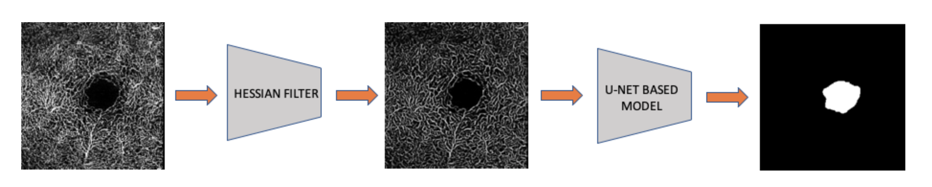
To address these limitations, we propose a hybrid pipeline that bridges traditional computer vision techniques with a modern U-Net-based model to automatically and accurately quantify the FAZ in OCTA images. First, we apply a Hessian-based filter to selectively enhance the blood vessels within the OCTA scans. We then feed these enhanced images into a specialized U-shape semantic segmentation model to extract the avascular zone. We demonstrate that this combined approach robustly outperforms traditional baseline methods, such as the Level Set, by a significant margin.
Methodology and Materials
Dataset
Two independent clinical datasets were used in this study. The primary dataset was provided by the Joseph Carroll Lab (Medical College of Wisconsin, Milwaukee, WI, USA) and consists of 230 OCTA images acquired from the superficial capillary plexus. Each image in this dataset was manually delineated by a single expert grader using ImageJ (National Institutes of Health, Bethesda, MD); further details on the acquisition protocol and grading procedure can be found in (Linderman et al., 2017). The second dataset was sourced from the Duke Eye Center and comprises 30 OCTA images of the deep vascular complex (DVC), representing a distinct imaging layer with different contrast and morphological characteristics.
The two datasets were split as follows: 184 images from the JC dataset for training, all 30 Duke images for validation, and the remaining 46 JC images held out as the test set. The Duke dataset was designated as the validation set because this configuration consistently yielded superior model performance — as measured by the Jaccard coefficient — compared to the reverse arrangement. Prior to being passed to the network, all images were enhanced by the Hessian-based filter described in the following section.
Hessian Filter
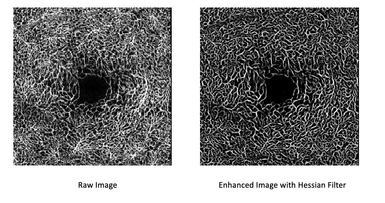
The Hessian filter analyzes the local second-order curvature of an image to detect and enhance tubular structures such as blood vessels, while suppressing blobs and flat backgrounds. We use the Frangi vesselness formulation (Frangi et al., 1998), which scores each pixel by how well its local geometry matches a tube-like shape across multiple scales. For a full conceptual and mathematical treatment, see the [Primer] Hessian Filter for Vessel Enhancement post.
Tuning the Scale - Practical Considerations for $\sigma$
The most critical parameter when deploying the Frangi filter is the Gaussian scale, $\sigma$. Because the algorithm relies on Gaussian smoothing before calculating the Hessian matrix, the value of $\sigma$ directly corresponds to the radius of the tubular structures you intend to extract.
When processing clinical data, in our case, isolating the microvasculature in OCTA scans, configuring $\sigma$ correctly is the difference between a clean extraction and a noisy mess. A small $\sigma$ (e.g., 0.5) sensitizes the filter to fine, delicate capillaries. A larger $\sigma$ (e.g., 2.5) shifts the focus to wider, primary vessels.
In practice, a single $\sigma$ is rarely sufficient. You must define a range ($\sigma_{min}$ to $\sigma_{max}$) that covers the expected anatomical variation in vessel radii within your specific imaging modality. The algorithm computes the vesselness score at multiple scales within this range and retains the maximum response for each pixel. An example of the filter applied to retinal OCT-A data is shown in Figure 1.
U-Net
Our segmentation model builds on the U-Net architecture (Ronneberger et al., 2015), a fully convolutional encoder–decoder network originally developed for biomedical image segmentation. The key idea of U-Net is its symmetric structure: a contracting encoder path that progressively captures high-level semantic context, paired with an expanding decoder path that recovers spatial resolution through up-sampling, with skip connections bridging the two halves to preserve fine-grained boundary details.
We depart from the original design by replacing the vanilla encoder with a SE-ResNeXt-50 backbone (Hu et al., 2019). SE-ResNeXt-50 combines the grouped convolutions of ResNeXt with Squeeze-and-Excitation (SE) blocks, which recalibrate channel-wise feature responses by explicitly modelling interdependencies between channels. This allows the encoder to produce richer, more discriminative feature maps while remaining computationally tractable. The decoder branch is then redesigned to progressively up-sample these encoded features back to full resolution, producing the final binary FAZ segmentation mask. Although other backbone architectures were explored, SE-ResNeXt-50 consistently yielded the best segmentation performance in our experiments.
The model was trained for 70 epochs with a batch size of 8, input resolution of 256 × 256, a learning rate of 0.0002, and the Adam optimizer.
Level Set
Originally introduced by Osher and Sethian (Osher & Sethian, 1988), the Level Set method has become a widely adopted tool in biomedical image segmentation owing to its capacity to represent and evolve boundaries of complex, irregular shapes. The core idea is to embed the segmentation contour as the zero level set of a higher-dimensional scalar function $\phi$, called the level set function (LSF). Rather than tracking the boundary explicitly, the algorithm evolves $\phi$ according to image-derived forces — typically based on intensity gradients — causing the zero contour to migrate toward and lock onto object edges.
In this study we use the Distance Regularized Level Set Evolution (DRLSE) formulation (Li et al., 2010), which augments the standard energy functional with a regularization term that penalizes deviations of $\phi$ from a signed distance function. This eliminates the need for periodic re-initialization — a costly and numerically error-prone step required by classical level set methods — and permits a broader and more robust class of initializations. To automate the method, we develop an intensity-based heuristic to place the initial contour, and then run the DRLSE evolution on Hessian-filtered images to identify the FAZ boundary. For a full conceptual and mathematical treatment, see the [Primer] Level Set Methods for Image Segmentation post.
<figure id=”fig-levelset-demo” style=”text-align:center”> <video autoplay loop muted playsinline style=”width:60%”> <source src=”/assets/img/FAZSEG/demo.mp4” type=”video/mp4”> </video>
</figure>
<figure style=”text-align:center”> <div style=”position:relative; padding-bottom:56.25%; height:0; overflow:hidden; max-width:100%”> <iframe src=”https://www.youtube.com/embed/amzJiJf-R0I” title=”Level Set method demonstration” frameborder=”0” allow=”accelerometer; autoplay; clipboard-write; encrypted-media; gyroscope; picture-in-picture” allowfullscreen style=”position:absolute; top:0; left:0; width:100%; height:100%”></iframe> </div>
</figure>
Evaluation
Jaccard Score
The Jaccard index (also known as Intersection over Union, IoU) measures the overlap between the predicted segmentation mask $\hat{S}$ and the ground truth mask $S$:
\[J(S, \hat{S}) = \frac{|S \cap \hat{S}|}{|S \cup \hat{S}|} = \frac{TP}{TP + FP + FN}\]where $TP$ is the number of true positive pixels, $FP$ is false positives, and $FN$ is false negatives. The score ranges from 0 (no overlap) to 1 (perfect agreement). It is stricter than the Dice coefficient because it penalizes both over- and under-segmentation symmetrically.
False Positive and False Negative
A false positive (FP) occurs when a pixel is predicted as FAZ but does not belong to the ground truth mask — the model over-segments into background or vessel regions. A false negative (FN) occurs when a pixel belongs to the ground truth FAZ but is missed by the prediction — the model under-segments the region. Both are normalized by the total ground truth area:
\[FP = \frac{|\hat{S} \setminus S|}{|S|}, \qquad FN = \frac{|S \setminus \hat{S}|}{|S|}\]A low FP indicates few spurious predictions; a low FN indicates good sensitivity to the full extent of the FAZ. Together with the Jaccard score, they provide a more complete picture of where a method tends to fail.
Results
Three configurations were evaluated: Hessian Filter + Level Set, U-Net alone, and the proposed Hessian Filter + U-Net pipeline. The first two serve as baselines — the Level Set baseline isolates the contribution of the deep learning component, while the standalone U-Net baseline quantifies the benefit of Hessian preprocessing. Quantitative results are reported in Table 1.
| Methods | Jaccard | FP | FN | |||
|---|---|---|---|---|---|---|
| Mean | STD | Mean | STD | Mean | STD | |
| Hessian + Level Set | 54.59 | 37.12 | 27.37 | 41.53 | 44.59 | 38.64 |
| Hessian + U-Net | 87.76 | 5.49 | 3.59 | 5.26 | 8.83 | 4.31 |
| U-Net | 86.49 | 9.63 | 9.17 | 9.53 | 5.17 | 4.62 |
The proposed Hessian Filter + U-Net pipeline achieved the highest mean Jaccard score (87.76%), outperforming both the standalone U-Net (86.49%) and the Hessian Filter + Level Set baseline (54.59%) by a wide margin. Beyond raw accuracy, the Hessian preprocessing had a pronounced effect on prediction consistency: the standard deviation of the Jaccard score dropped from 9.63% for U-Net alone to 5.49% with preprocessing, indicating that the filter produces cleaner, more structured input that the network can segment more reliably across diverse cases. The proposed method also recorded the lowest mean FP (3.59%) and the lowest standard deviations for both FP and FN, suggesting that its predictions are not only accurate on average but also tightly concentrated around that average. Representative segmentation outputs are shown in Figure 4.
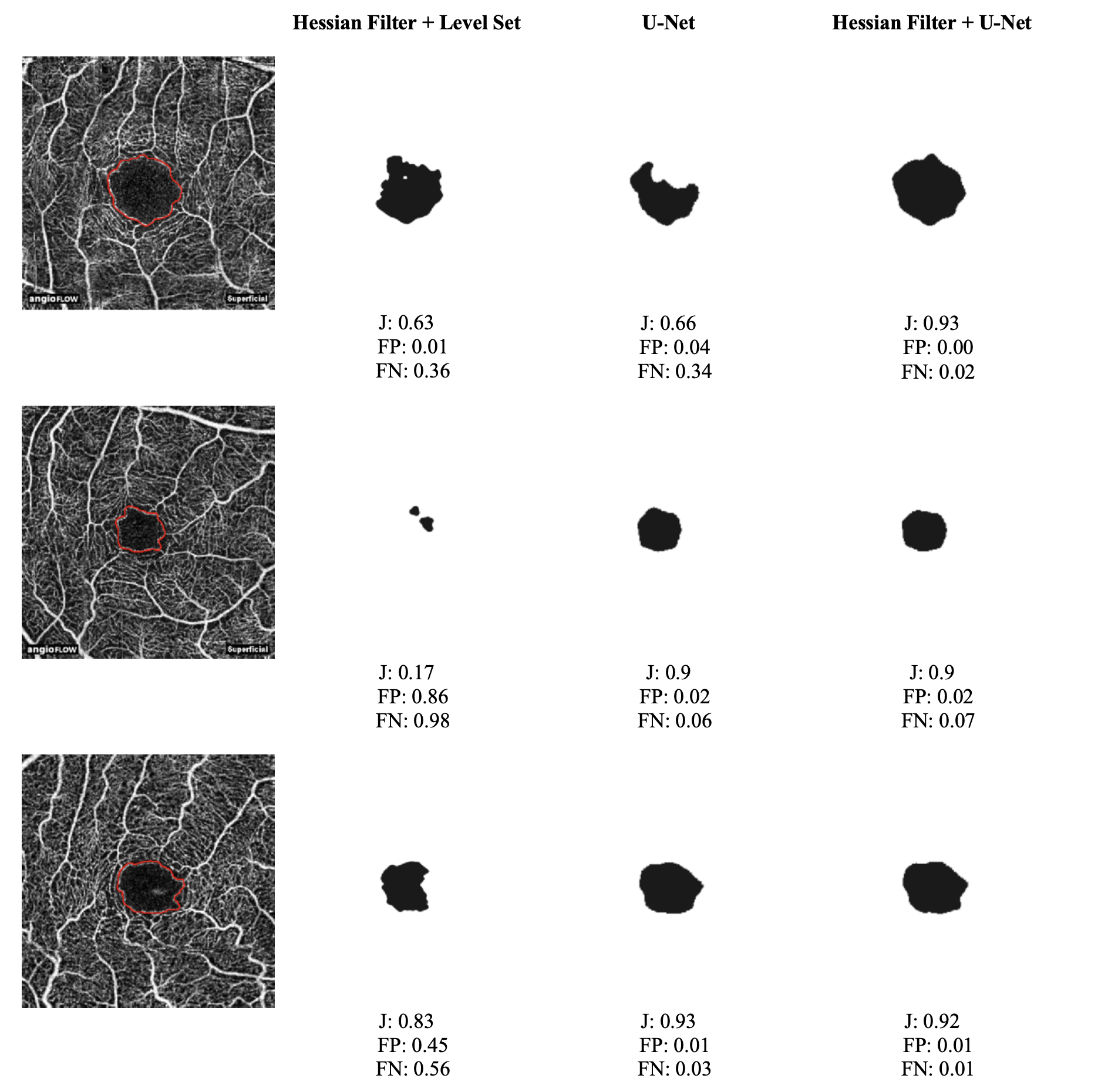
The Level Set baseline performed poorly overall, with a mean Jaccard of only 54.59% and an extremely high variance (STD 37.12%), reflecting frequent segmentation failures rather than a consistent but inaccurate result. Two factors likely account for this. First, the low imaging resolution (304 × 304 pixels) combined with heavy intra-FAZ noise makes it difficult for gradient-based contour evolution to distinguish true FAZ boundaries from noise artifacts, causing the contour to stall or collapse prematurely. Second, the initial contour was hard-coded to the image center, which is problematic in practice since the FAZ is not always centered in the field of view. A misplaced initialization can trap the contour in a local energy minimum far from the true boundary, a failure mode that deep learning avoids entirely by learning a global feature representation of the region.
Conclusion
This study demonstrates that deep convolutional neural networks are a highly effective tool for FAZ segmentation in OCTA images. Even when trained on a relatively small dataset, the SE-ResNeXt-50-based U-Net substantially outperformed the Level Set baseline, a classical technique that remains widely used in clinical image analysis, across all three evaluation metrics. This gap underscores the ability of deep networks to learn robust, data-driven representations that generalize across the anatomical and imaging variability inherent in clinical OCTA data, without requiring hand-tuned initialization or manual parameter selection.
Beyond the core architecture, the results confirm that Hessian-based preprocessing provides a meaningful and consistent benefit. By enhancing the vascular contrast of the input images prior to segmentation, the filter supplies the network with cleaner, more structured input, which translates into higher mean accuracy and, crucially, a tighter distribution of predictions across samples. The reduction in Jaccard standard deviation, from 9.63% for U-Net alone to 5.49% with Hessian preprocessing, suggests that the filter mitigates the effect of low-quality or noisy scans that would otherwise destabilize the model’s output.
One aspect that warrants further investigation concerns the choice of validation set. During training, we observed that using the Duke dataset for validation and the JC dataset for testing yielded a noticeably better final model than the reverse split. Because neither the validation nor the test set contributes to gradient updates, this asymmetry is not immediately explained by standard overfitting arguments. One plausible hypothesis is that the Duke and JC datasets differ subtly in image acquisition protocol, contrast characteristics, or FAZ morphology distribution, causing the validation loss landscape to differ between the two splits in ways that affect early stopping and learning rate scheduling. Characterizing these inter-dataset differences more rigorously, and developing validation strategies that are robust to them, remains an important direction for future work.
References
2020
- Improved Automated Foveal Avascular Zone Measurement in Cirrus Optical Coherence Tomography Angiography Using the Level Sets MacroTranslational Vision Science & Technology, 2020
2019
- Automatic segmentation of the foveal avascular zone in ophthalmological OCT-A imagesPLOS ONE, 2019
- Squeeze-and-Excitation NetworksIEEE Transactions on Pattern Analysis and Machine Intelligence, 2019
2018
- Evaluation of Automatically Quantified Foveal Avascular Zone Metrics for Diagnosis of Diabetic Retinopathy Using Optical Coherence Tomography AngiographyInvestigative Ophthalmology & Visual Science, 2018
2017
- Assessing the Accuracy of Foveal Avascular Zone Measurements Using Optical Coherence Tomography Angiography: Segmentation and ScalingTranslational Vision Science & Technology, 2017
2015
- A review of optical coherence tomography angiography (OCTA)International Journal of Retina and Vitreous, 2015
- Optical coherence tomography (OCT) for detection of macular oedema in patients with diabetic retinopathyCochrane Database of Systematic Reviews, 2015
- U-Net: Convolutional Networks for Biomedical Image SegmentationIn Medical Image Computing and Computer-Assisted Intervention — MICCAI 2015, 2015
2014
- Quantitative optical coherence tomography angiography of choroidal neovascularization in age-related macular degenerationOphthalmology, 2014
2010
- Distance Regularized Level Set Evolution and Its Application to Image SegmentationIEEE Transactions on Image Processing, 2010
1998
- Multiscale vessel enhancement filteringIn Medical Image Computing and Computer-Assisted Intervention — MICCAI’98, 1998
1988
- Fronts propagating with curvature-dependent speed: Algorithms based on Hamilton-Jacobi formulationsJournal of Computational Physics, 1988